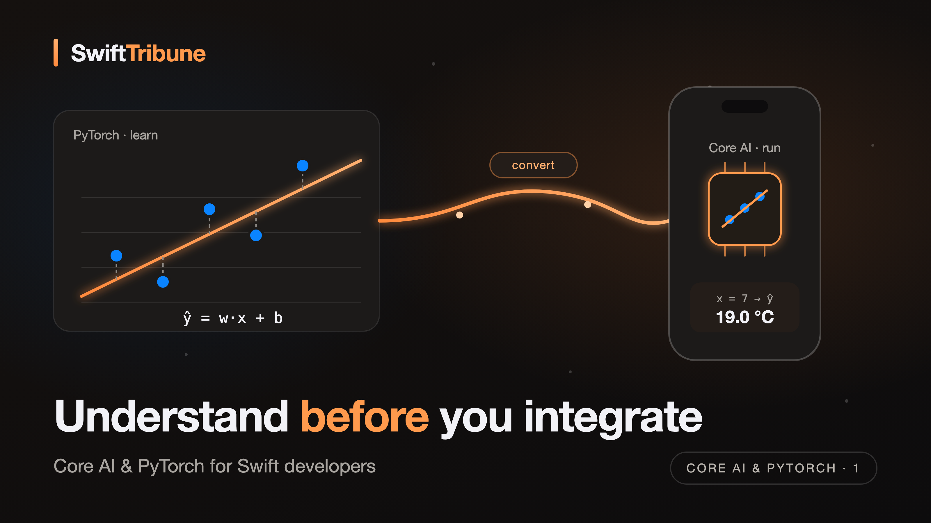
Introduction
An AI agent can now write a PyTorch model and convert it to Core AI in a few minutes. So why should a Swift developer still learn how that model works? This series is my answer, and it starts with the basics.
It comes from a very concrete shift in our ecosystem. Since WWDC 2026, Apple has adopted Core AI as the way to bring models into our apps. For Swift developers, the question is no longer only which API to call. We also have to ask where the model comes from and what exactly we are shipping. More and more often, the answer starts in Python, with a model built and trained in PyTorch long before it reaches Xcode.
As Swift developers, we can now ask Claude or ChatGPT to generate a model in Python, prepare its training with PyTorch, and even walk us through the conversion to Core AI. Work that used to take specialised knowledge and several hours can now be done much faster.
But one question deserves to be asked.
Do we actually understand what we are building?
I don’t think copy-paste was born with AI. We have always pulled code from Stack Overflow, GitHub or technical blogs. We have all reused a solution found online to fix a problem, sometimes without understanding every line.
What has changed is mostly the time it takes to get an answer.
We used to spend twenty minutes on Stack Overflow, reading several answers and trying to find the one that matched our situation. Today we ask Claude or ChatGPT and get an answer adapted to our context in a few seconds.
The experience is different too. We can ask the same question several times, ask for a simpler explanation, come back to a concept or try another approach. The AI never gets impatient, and it never makes us feel that our question is stupid.
I find this evolution really interesting. It makes learning much more accessible.
It doesn’t remove a risk we already know well, though. We can simply replace copy-pasting a Stack Overflow answer with copy-pasting an answer generated by Claude. The result comes faster and often fits our context better, but our understanding hasn’t necessarily moved.
The developer’s role is changing, but reasoning still matters
I am not here to judge whether we should use AI for this kind of work. That debate is over. AI is part of how we build software now, it’s a fact. I don’t think we should stop delegating work to it. We should learn to use it better.
What worries me is something else. I don’t want a Swift developer to ask an AI to write an LLM in PyTorch, convert it and ship it without understanding how the engine works underneath. Using a tool you don’t understand is fine until the day it breaks, and with Machine Learning that day always comes.
Today an agent can generate an architecture, write tests, fix errors, build a Machine Learning model and automate part of its integration into an app.
But when something goes wrong, can we understand what happened?
Imagine we ask an agent to build a PyTorch model and then convert it to Core AI. The conversion fails. If we know nothing about the model’s architecture, its tensors or the operations it uses, we will probably paste the error message back into the chat and wait for a new answer.
Maybe it will find a fix. Maybe it will propose a change that hides the problem without solving it.
If we understand the fundamentals, we can ask more precise questions, check its assumptions, push back on its proposals and judge the consequences of its changes.
We don’t need to become experts in every technology we use. We do need enough knowledge to understand what we are building and to keep our own judgement.
That is the idea behind this series, and it’s why it covers two worlds. PyTorch is where a model is born, where it gets defined, trained and understood. Core AI is where it lives in our apps, converted, optimised and run on Apple devices from Swift. Knowing PyTorch without Core AI leaves the model stuck on a Mac. Knowing Core AI without PyTorch means shipping a black box.
So I don’t only want to show how to ask Claude for a PyTorch model and how to convert it to Core AI. I want to understand what happens between those two steps. I want to be able to read the generated code, follow what the conversion does to it, and ask the right questions when something doesn’t work.
AI can speed up our work a lot. It shouldn’t stop us from thinking.
A personal note, this one took months
Writing this series took me months. My previous series, on Apple’s Evaluations framework, already took my whole summer. This one took longer, and understanding it was painful at times.
The paradigm changed for me. As an iOS developer, I spent years writing rules, with functions, state and control flow. Machine Learning asks you to think differently. You no longer describe the solution. You describe how wrong you are, and an algorithm reduces that error. It took me a while to really absorb that, and I suspect I’m not the only one.
Along the way I realised that a solid mathematical base matters much more than I expected. Not to become a researcher, but to understand why things are done the way they are. Why do we use derivatives to train a model? What is a linear equation, exactly? What does it mean for a function to have several parameters and several inputs? Without those answers, PyTorch code reads like a list of incantations. With them, every line has a reason to be there.
None of this is hard. It just asks for some effort. That’s why this first part spends real time on the maths, one small step at a time, always with actual numbers. If you take the time to follow it, the rest of the series will be much easier to read.
Why start with PyTorch?
When we work in the Apple ecosystem, it’s tempting to jump straight to the tools in Xcode and the frameworks that run models on Apple devices.
Before integrating a model, though, we need to understand what it represents and how it was built. That’s where PyTorch comes in.
PyTorch is one of the most widely used frameworks to build, train and experiment with Machine Learning models. It lets us manipulate data, define neural network architectures, measure errors and train models.
We are not trying to become PyTorch specialists. We will use it as a concrete way to understand how a model works. Then the series will follow that same model into Core AI and into a Swift app. PyTorch to understand and build it, Core AI to integrate and run it.
We’ll start from a deliberately simple problem, and this time we won’t skip the few equations that make it click. They are short, and each one maps to a line of code you’ll write in Part 2.
1. Writing a rule or learning from data
Imagine we want to estimate the outside temperature from a sunshine index.
With a traditional approach, we could write a Swift function like this one.
func predictTemperature(sunshineIndex: Double) -> Double {
    return 2 * sunshineIndex + 5
}
Nothing surprising here. We defined a formula, and the program applies it every time it receives a new value. If the sunshine index is 3, the function returns 11.
The program doesn’t try to discover a relationship. It runs exactly the instructions we wrote.
Machine Learning takes a different approach. We have a set of past observations, and for each one we know the sunshine index and the temperature that was actually measured.
| Sunshine index | Observed temperature |
|---|---|
| 1 | 7 °C |
| 2 | 9 °C |
| 3 | 11 °C |
| 4 | 13 °C |
| 5 | 15 °C |
We give these examples to a model and ask it to learn the relationship between the two values. We never give it the formula. It adjusts its parameters from the data so that it can produce predictions.
Once trained, the model can receive a new value, say a sunshine index of 7, and estimate the temperature.
In this teaching example the data follows a deliberately clean relationship. In a real problem, relationships are usually more complex and the observations contain noise.
That’s the fundamental difference.
In traditional development, we write the rules. In Machine Learning, we provide data and the model learns the rule.
2. What is a model?
A Machine Learning model is a parameterised mathematical function. It turns input data into results using internal parameters.
In our example, the simplest model we can pick is a straight line.
Each symbol has a precise role, and you’ll meet all of them again in PyTorch.
- is the input, here the sunshine index.
- , read “y-hat”, is the prediction, the temperature the model thinks it is. The hat always means “estimated”.
- is the weight. It says how much the temperature changes when the sunshine index goes up by one.
- is the bias, the baseline temperature when the sunshine index is zero.
Together, and are the model’s parameters, often written as a single symbol . Our Swift function from section 1 is exactly this model, with the parameters fixed by hand at and .
With Machine Learning, nobody types the 2 and the 5. The model starts with arbitrary values and adjusts them during a phase called training. At first its predictions can be far from reality. Step by step, it changes its parameters to reduce the gap between its predictions and the observed temperatures. That process is what we call learning.
In Swift, the model looks less like a function and more like a struct with mutable state.
struct LinearModel {
    var weight: Double   // w, learned
    var bias: Double     // b, learned

    func callAsFunction(_ x: Double) -> Double {
        weight * x + bias
    }
}

var model = LinearModel(weight: 1, bias: 0)   // an untrained guess
model(3) // 3.0, far from the 11 °C we observednn.Linear(1, 1), with one input, one output, one weight and one bias. When you see nn.Linear in generated code, you now know it computes and nothing more.The model doesn’t understand temperature the way we do. It learns a mathematical representation of the relationships in the data, and reuses it to predict new observations. Image classifiers and language models have millions or billions of parameters instead of two, but the principle is the same.
3. Features and labels
To understand how a model learns, we first need to look at the data we give it. Supervised Machine Learning relies on two notions.
- Features are the pieces of information the model uses to make a prediction.
- Labels are the expected results, the ground truth.
In our example, the sunshine index is the feature and the observed temperature is the label.
| Feature | Label |
|---|---|
| 1 | 7 °C |
| 2 | 9 °C |
| 3 | 11 °C |
| 4 | 13 °C |
| 5 | 15 °C |
Take the first observation, with feature and label . It means we measured 7 °C when the sunshine index was 1.
In mathematical terms, the whole dataset is a set of pairs, and the subscript identifies one observation.
During training, the model receives the feature and produces its own prediction . We then compare that prediction with the label to measure its error.
Features give the model what it needs to predict. Labels tell us whether the result is close to what we expect.
More than one feature
In a real project, a model usually receives several features. To estimate a temperature we might use sunshine, humidity, atmospheric pressure and wind speed. Each feature gets its own weight.
Here the subscript counts the features, not the observations. One observation is now a list of four numbers, a vector, and the whole dataset becomes a table of numbers with one row per observation and one column per feature. In PyTorch those tables are called tensors, and they are the topic of Part 2.
4. Supervised learning and the loss function
The example we just built belongs to a category called supervised learning. We give the model examples for which we already know the expected result, so every observation contains features and a label.
The model uses the features to produce a prediction, and we compare that prediction with the matching label. The comparison gives us the model’s error, and during training that error is used to adjust its parameters.
“Measure the error” deserves more than a box in a diagram, because it is the heart of training. We’ll go through it in three steps.
The error of one prediction
For one observation, the error, also called the residual, is the gap between what the model predicted and what was observed.
Let’s take our untrained model, with and , and run it on the five observations.
| label | prediction | error | ||
|---|---|---|---|---|
| 1 | 7 | 1 | −6 | 36 |
| 2 | 9 | 2 | −7 | 49 |
| 3 | 11 | 3 | −8 | 64 |
| 4 | 13 | 4 | −9 | 81 |
| 5 | 15 | 5 | −10 | 100 |
Every error is negative, so the model predicts temperatures that are far too low.
One number for the whole dataset
To improve, the model needs a single number that tells it how wrong it is overall. We can’t just add the errors, because a +5 and a −5 would cancel out and make the model look perfect. So we square each error first, which also punishes big mistakes much more than small ones, and then take the average. This is the Mean Squared Error, or MSE.
This function is called the loss function. Look at what it depends on. The data doesn’t change, so the loss only depends on and . Training means finding the and that make it as small as possible.
For our untrained model, we get 66.
With the “true” parameters and , every prediction matches its label and every error is zero, so . That’s the target.
Here is the same calculation in Swift.
func meanSquaredError(model: LinearModel, data: [(x: Double, y: Double)]) -> Double {
    let squaredErrors = data.map { sample in
        let error = model(sample.x) - sample.y
        return error * error
    }
    return squaredErrors.reduce(0, +) / Double(data.count)
}

let data: [(x: Double, y: Double)] = [(1, 7), (2, 9), (3, 11), (4, 13), (5, 15)]
meanSquaredError(model: LinearModel(weight: 1, bias: 0), data: data)  // 66.0
meanSquaredError(model: LinearModel(weight: 2, bias: 5), data: data) // 0.0nn.MSELoss(). When an agent writes loss_fn = nn.MSELoss(), it’s the formula above and nothing else.Which way to move, a first look at gradient descent
We know how wrong the model is. How does it know in which direction to change and ?
This is where derivatives come in. The derivative of the loss with respect to a parameter tells us how the loss changes when we nudge that parameter a little. For the MSE, the two derivatives, together called the gradient, look like this.
You don’t need to derive them yourself. For , you take each error, multiply it by its input, add everything up and scale the result. For , you do the same without the multiplication. A negative gradient means that increasing the parameter would lower the loss.
Then we take a small step in the opposite direction of the gradient. This is gradient descent.
The symbol , eta, is the learning rate, the size of each step. The model doesn’t learn it, we choose it. Values like this one, which configure the training instead of being learned by it, are called hyperparameters.
Let’s do one step by hand, starting from and with . We already have the errors .
Both gradients are negative, so both parameters go up.
If you compute the loss again with these new parameters, you get . After a single step, the error went from 66 to about 40. Repeat the loop a few thousand times and the parameters end up at and . The model found the formula we never gave it.
Try it yourself
The playground below runs exactly these equations. Move the sliders to fit the line by hand and watch the dashed errors and the MSE change. Then press “One gradient step” a few times, or “Train”, and watch the loss curve go down.
Train the model yourself
Move w and b by hand, or let gradient descent do it. The goal is to make the MSE as small as possible.
MSE over training steps
Two experiments are worth trying.
- Fit the line by hand first. You’ll quickly notice that and depend on each other. When you change one, the best value for the other moves too. That’s why we need the gradient, which takes both into account at once.
- Set and press “Train”. This time the model diverges. Each step overshoots the minimum a bit more than the previous one, and the loss explodes. A badly chosen learning rate is one of the first things that goes wrong in real training, and now you’ll recognise the symptom when you see
loss: nanin a training log.
loss.backward() computes the gradient for you (the feature is called autograd), and an optimizer such as torch.optim.SGD(model.parameters(), lr=0.05) applies the update. We’ll write that loop line by line in Part 2.5. Regression and classification
Machine Learning models don’t all produce the same kind of result. Two big families of problems show the difference.
Regression
We use regression when we want to predict a numeric value. Our temperature example is a regression problem. The model can predict 18.5 °C, 21 °C or 24.3 °C, any value on a continuous scale. That’s why we leave the output of our model, , as it is. It can be any real number.
A few other examples.
- Predicting the price of a home.
- Estimating the electricity consumption of a house.
- Predicting how long a trip will take.
Classification
We use classification when we want to assign a category to an observation. Imagine we want to know whether an image shows a cat or a dog. The model receives an image and has to identify the right category.
A few other examples.
- Detecting whether an email is spam.
- Flagging a transaction as suspicious or normal.
- Recognising the type of object in a picture.
Under the hood, a classifier still computes numbers. The difference is that its raw output gets squashed into a probability between 0 and 1. For a yes or no question, the usual tool is the sigmoid function.
If for an email, the model is saying “92% spam”. We then pick a threshold, often 0.5, to turn that probability into a category. Since the output is now a probability, the MSE is no longer the right way to measure the error. Classifiers use another loss called cross-entropy, which we’ll see later in the series.
| Regression | Classification | |
|---|---|---|
| Output | A number, e.g. 19.0 °C | A category, e.g. “spam” |
| Last step of the model | Nothing, raw value | Sigmoid / softmax → probabilities |
| Typical loss | Mean squared error | Cross-entropy |
| PyTorch | nn.MSELoss() |
nn.BCEWithLogitsLoss(), nn.CrossEntropyLoss() |
As an iOS developer, this difference tells you what the model’s output means once it reaches your Swift code. A regression model gives you a value to display. A classifier gives you probabilities that you have to interpret.
6. Training and inference
One last distinction before we move to PyTorch. Training and inference are two different phases in the life of a model.
Training
During training, the model learns from data. It receives features, produces predictions, compares them with labels and gradually adjusts its parameters to reduce its errors. It’s the loop from section 4, repeated over the whole dataset many times. Each full pass over the data is called an epoch.
This phase can need a lot of computation. Large models train on powerful GPUs for hours or weeks.
Inference
Inference happens after training. The model uses the parameters it learned to make predictions on new data. There are no labels, no loss and no gradient, only the forward computation.
Back to our example, we trained on these observations.
1 -> 7 °C
2 -> 9 °C
3 -> 11 °C
4 -> 13 °C
5 -> 15 °C
Training found and . Now we ask for a sunshine index of 7.
In this phase the model doesn’t need the real temperature to make its prediction. It just uses the parameters it learned. You can see this point on the right side of the playground above, in the “inference” zone.
| Training | Inference | |
|---|---|---|
| Goal | Find good parameters | Use the parameters |
| Needs labels? | Yes | No |
| Computes loss and gradients? | Yes | No |
| Parameters | Change at every step | Frozen |
| Where it usually runs | Python, PyTorch, GPUs | On device, in your Swift app |
This distinction matters a lot for iOS developers. In many projects, we take a model that is already trained, convert it into a format Apple’s frameworks understand, and run it from our Swift app. What you ship to the device is the frozen parameters plus the forward computation, not the training loop.
So we are not necessarily responsible for training. We do need to understand the model well enough to know what it expects as input, what it returns, and how to check that it behaves correctly.
Conclusion
Before writing any PyTorch code, we laid the foundations to understand what a Machine Learning model is.
We saw the difference between a traditional function, which applies the rules we wrote, and a model, which learns its rule from examples. A model is a function with parameters, here , and training is the process that finds good values for and . Features are the inputs, and labels are the ground truth we compare the predictions with. The MSE turns “how wrong is the model?” into a single number. The gradient tells us in which direction to move each parameter, and the learning rate tells us how far. Regression predicts a number, classification predicts a category through probabilities. And training is where parameters are learned, while inference is where they are used, very often on the device.
These ideas can look theoretical, but each of them maps to a line of PyTorch you’ll soon read and write. The goal isn’t to become Machine Learning experts. It’s to understand enough to know what we are manipulating, to work well with AI agents, and to keep our judgement.
If you only remember three things from this part, keep these.
- A model is a function with parameters, and training only searches for good values of those parameters.
- The loss turns “how wrong is the model?” into one number, and the gradient says which way to move to make it smaller.
- What you ship in your app is inference, the learned parameters and the forward computation, not the training.
In the next part we move to practice with PyTorch. We’ll start with tensors, then build our first regression model to predict a temperature, and you’ll recognise every equation from this article in the code. After that, we’ll take this same model to Core AI and run it from Swift, so that nothing between the first equation and the first on-device prediction stays a black box.
Before you go, open the playground again and try to reach an MSE below 1 by hand, without pressing “Train”. It’s the best way to feel what the gradient does for you. If something in this part wasn’t clear, or if you want me to go deeper on a topic, send me a message. Your questions will shape the next parts of the series.